Evictions of Alachua County (updated Dec 2022)
This is an update/revision/revamp to a previous post I made for my Urban Spatial Analysis class at UF. I revised a lot of methodology, analysis, and presentation of the same dataset used in the previous post.
The original project was prompted by some research interests as a Housing Campaign Coordinator at the Alachua County Labor Coalition. I ultimately finished my report on twenty years of evictions (a report I now perceive as an early draft) in summer of 2022 as my final for the Urban Spatial Analysis class. Here I analyze the 20 years of eviction and propose the following questions:
- Where do evictions occur in Alachua County?
- How do eviction-prone areas cluster and how do they act as outliers?
- What are the social and built environments of these areas? Can social and built environment predict evictions?
In the future, I hope to augment this page by adding a combined spatio-temporal component to my analysis.
Background and descriptions of the data
The ultimate source of the Alachua County Evictions 2002-2021 dataset is the Alachua County Clerk of Court. I used a pre-made web scraper directed at the case record search to acquire information about filings, including addresses. The original source is available on the Clerk of Court website. Acquired in January 2022, these data range from 2002-01-01 to 2021-12-31 and represent 34970 eviction filing over 20 years.
Using a custom built geocoder in R with the help of tidyverse and postmastr libraries, as well as Alachua County's E911 records and historical address crosswalk tables, I successfully geocoded 31770 eviction filings to at least the main address of a parcel. Using 2021 American Community Survey and 2020 census data, I joined data variables representing population, race and ethnicity, income, home ownership, householder, age and type of housing, poverty status and level, and receipt of public assistance to census block groups to create aggregation polygons for the evictions.
I ran a few descriptive statistics on the non-aggregated eviction locations. The county center by geography is located between NW 16th Ave and Glen Springs Blvd on NW 23rd Ter. By population according to the block groups, the center is located further southwest near NW 43rd St and NW 13th Ave. Evictions skew further southeast compared to that, finding their center at SW 34th St and SW 2nd Ave. This suggests that evictions are disproportionately heavier compared to the population somewhere in the east side of the county, be it East Gainesville or Hawthorne.
Use the map below to scroll through the descriptions of centers (find the legend button in the top left corner of the app). Behind the distribution, you'll also find the same kernelized distribution of evictions.
Clustering and Outliers
In my original report I switched between a few different modes of analyses - Getis-Ord Gi* (optimized and not), Global Moran's I, etc. I found the one that fit my data description needs most was the Optimized Outlier Analysis (OOA) which uses Anselin Local Moran's I and machine-learning techniques to find an optimized description of the data. Using the OOA, I also added two new parameters to explore effects on the data: whether I used hexagon aggregation of raw eviction counts or block group aggregation followed by a normalizing log-transformation, and whether I split the data between urban and rural scales, or analyzed the entire dataset together. Similar to the original draft, I omitted block groups representing UF campus because they were huge skewing outliers in the data (as well, legal evictions aren't the UF process in removing students from dormitories).
The justification for splitting the data into urban and rural scales lies in the methodology of Anselin Local Moran's I. It relies on calculating each features difference with its neighbors as well as the global mean. Gainesville holds the vast majority of evictions in the county, and in general urban areas have higher eviction levels than rural areas. By consideration of the entire dataset, any local hotspots or coldspots in rural areas are likely to be overshadowed by comparison to the global mean due to Gainesville.
When aggregating by hexagons and splitting between Gainesville and the county, two major high-eviction clusters emerge in a small band surrounding Alachua and a band in Gainesville from Holly Heights and Sparrow Condomiums to Phoenix and SW 35th Place. Low eviction outliers surround those bands. There are isolated high-eviction outliers mostly in Gainesville, and major low-eviction clusters in Northwest Gainesville, around Fort Clarke Boulevard and West Newberry Road, Haile and Arredondo, and isolated in rural Alachua County.
When aggregating by hexagons without splitting the data, the pattern becomes less clear. All of rural Alachua County becomes a low-low cluster while southwest and east Gainesville become high-high clusters. At the scale of the data, the low-low eviction cluster in northwest Gainesville becomes a low-high outlier.
When aggregating by block group with splitting the data, a lot of the clustering disappears except the northwest Gainesville low-eviction cluster and an odd single hotspot representing Butler Plaza in Gainesville.
When aggregating by block group without splitting, a band of block groups from Archer to La Crosse becomes a low eviction cluster with a high outlier northeast of Newberry. Most of east and southwest Gainesville emerges as high eviction clusters, with low outliers surrounding those block groups, especially in northwest Gainesville.
Overall, separating the dataset between rural and urban scales is a good way of localizing patterns to certain scales, ensuring that eviction levels impactful at one scale are not overshadowed or shadow another scale.
Modelling evictions
Lastly, to explore the ability of certain variables to predict evictions, I used the block group aggregations and census data to run exploratory regressions. I looked at data representing race and ethnicity, income, home ownership, householder, age and type of housing, poverty status and level, and receipt of public assistance to draw patterns. I limited my search of variables to those with 3-4 variables, and selected models that balanced explaining power with limited variables.
Out of 46937 models tested, the following variables were significant more than 90% of the time. (+/- means as the variable in question increases, evictions increase or decrease respectively).
- Proportion of population white and non-Hispanic/Latine (-)
- Proportion of population renting (+)
- Single-family detached housing (-)
- Single-family attached housing (+)
- Married couple-headed households (-)
- 3-4 unit housing (+)
- Single-female householder (+)
- Black or African American (+)
- Median household income (-)
- 5-9 unit housing (+)
In general, age of housing, other racial characteristics, and single male householders were not particularly useful in predicting evictions.
The top model of one variable was:
- -White (R² = 0.53, AICc = 400.85)
The top model of two variables was:
- -Single-family detached, -White (R² = 0.70, AICc = 340.48)
The top three models of three variables were:
- +Single-family attached, -Single-family detached, -White (R² = 0.72, AICc = 332.76)
- +Black/AA, +SF attached, -SF detached (R² = 0.71, AICc = 333.77)
- +Black/AA, -SF detached, +3/4 structure (R² = 0.71, AICc = 334.80)
The top three models of four variables were:
- +Black/AA, +Renters, +SF attached, -SF detached (R² = 0.73, AICc = 326.37)
- +SF attached, -SF detached, -Built 1990s, -White (R² = 0.73, AICc = 328.33)
- +Black/AA, +SF attached, -SF detached, -White (R² = 0.73, AICc = 328.73)
I chose the top model of three variables to explore (in bold). In theory I could've chosen the more generalizable two-variable model, but the three-variable gave just the right amount of complexity to the model.
Digging in
The full model can be represented by the equation Log(evictions) = 7.663 + 4.9783 * Single-family attached - -1.4342 * Single-family detached - 4.6145 * White. The model predicts that as the proportion living in single-family attached housing increases, so too will evictions. In contrast, the more people that are white and/or live in single-family detached housing, evictions will be predicted to decrease. Specifically in terms of magnitude, if you wanted to figure out how much a 10% change in a variable affects evictions, you take a tenth of the coefficient and have it be the exponent to an e base. Multiply the result by 100% and you get the percentage effect on evictions. For example, a 10% increase in the white population is predicted to correlate with a decrease of 37% in evictions.
One additional factor to add in is the role of space in this model - do the factors listed above have varying magnitudes of effects across the space of the dataset? I used Geographically Weighted Regression to figure this out. A summary of the residuals of both the non-spatial and spatial case follows.
Using the geographically weighted regression, I find that the raw R² jumps to 0.74 (from 0.72), so not much more fit was achieved from considering spatial effects. However, there were interesting outcomes from the data:
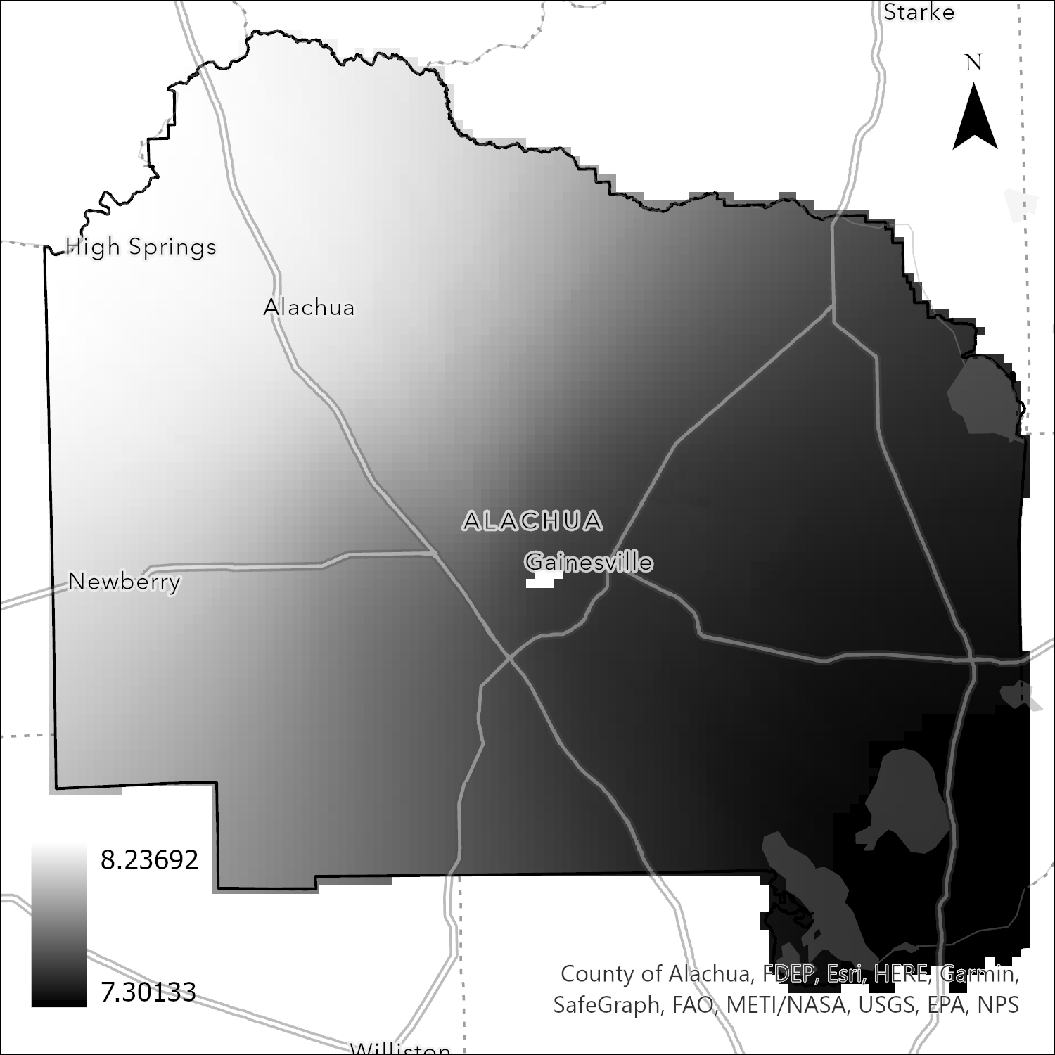
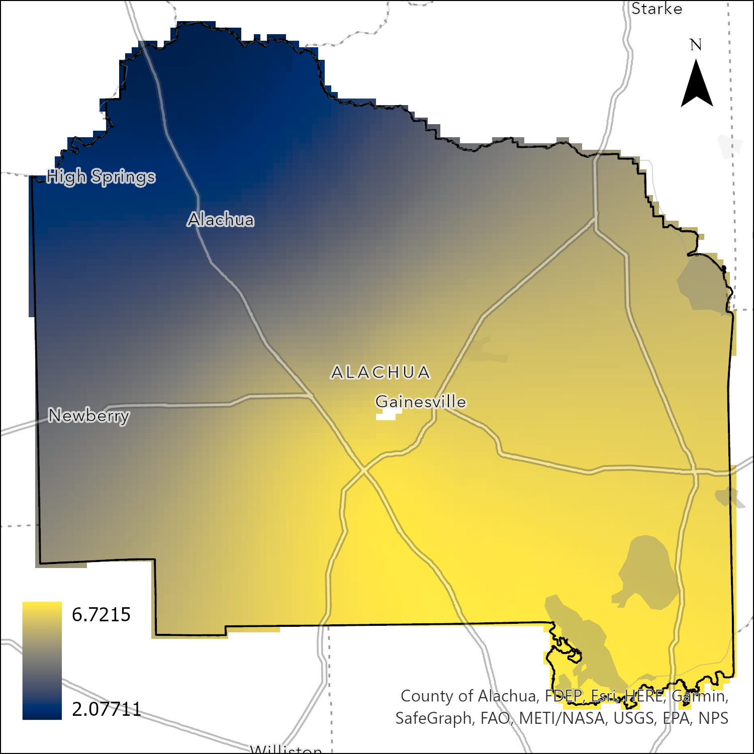
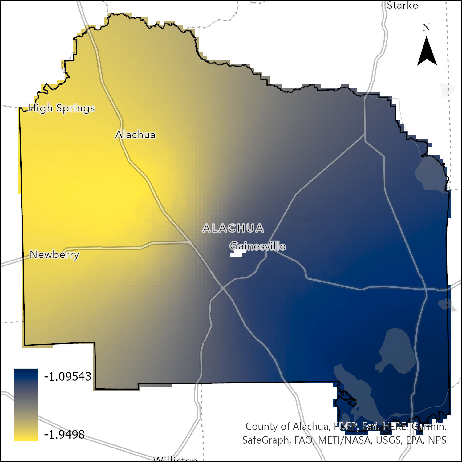
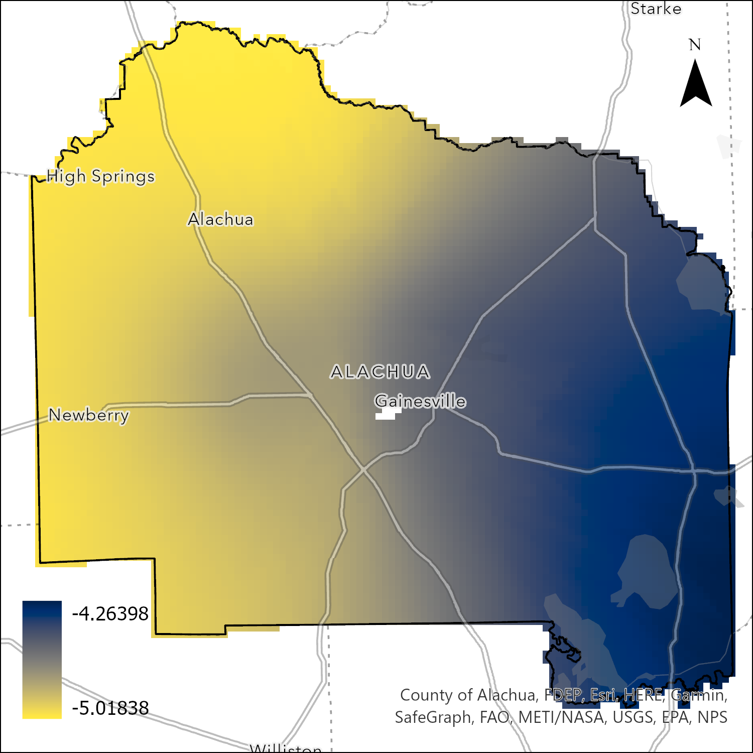
Whereas most model parameters varied no more than 1 across the county, the most drastic variation across the county belongs to the single-family attached coefficient which scales 4 magnitudes from northwest to southeast. Whereas a 10% increase in single-family housing in the northwest predicts a 122% rise in evictions, the same in the southeast predicts a 195% rise in evictions. Overall, the explaining power is only slightly increased by including the effect of space in the model.
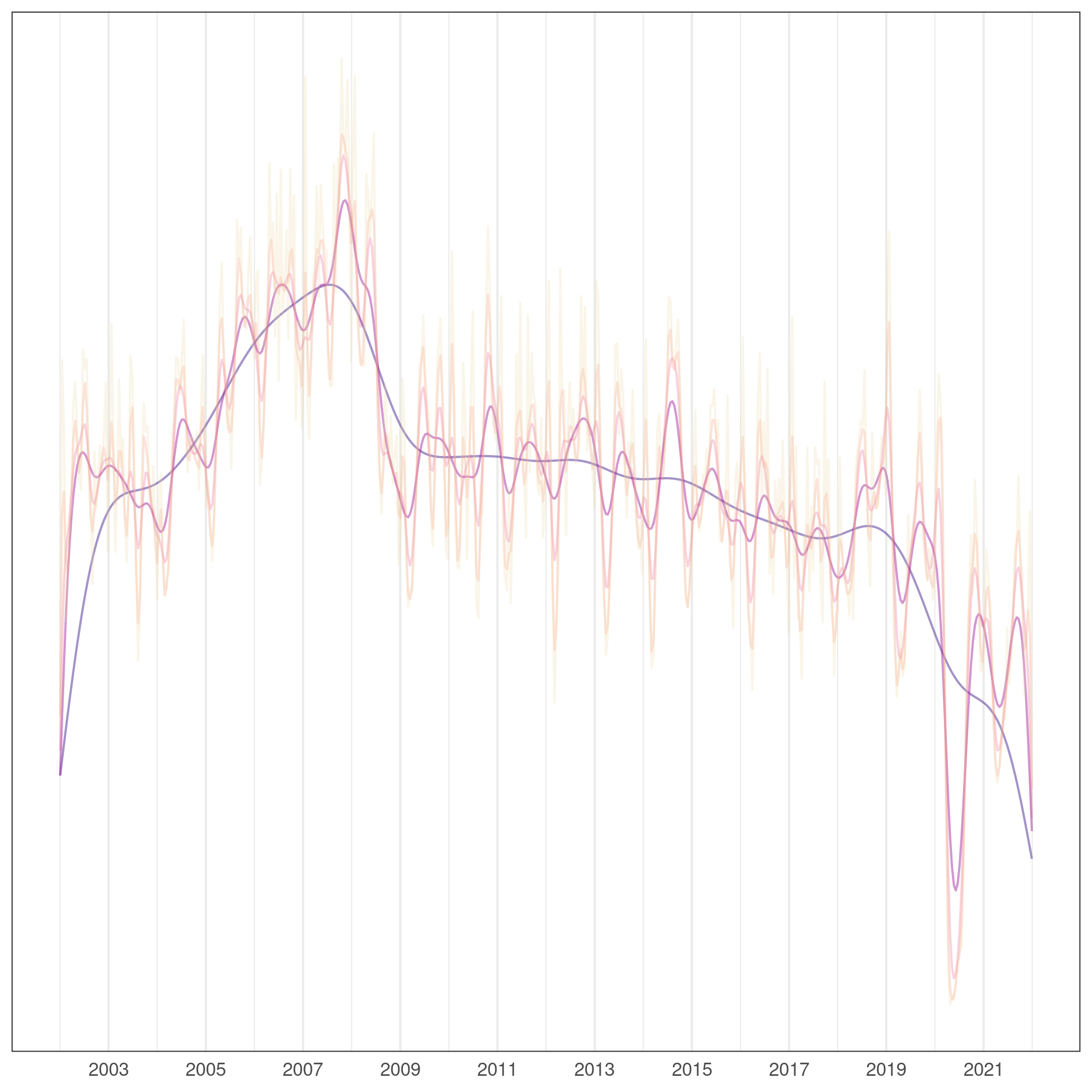
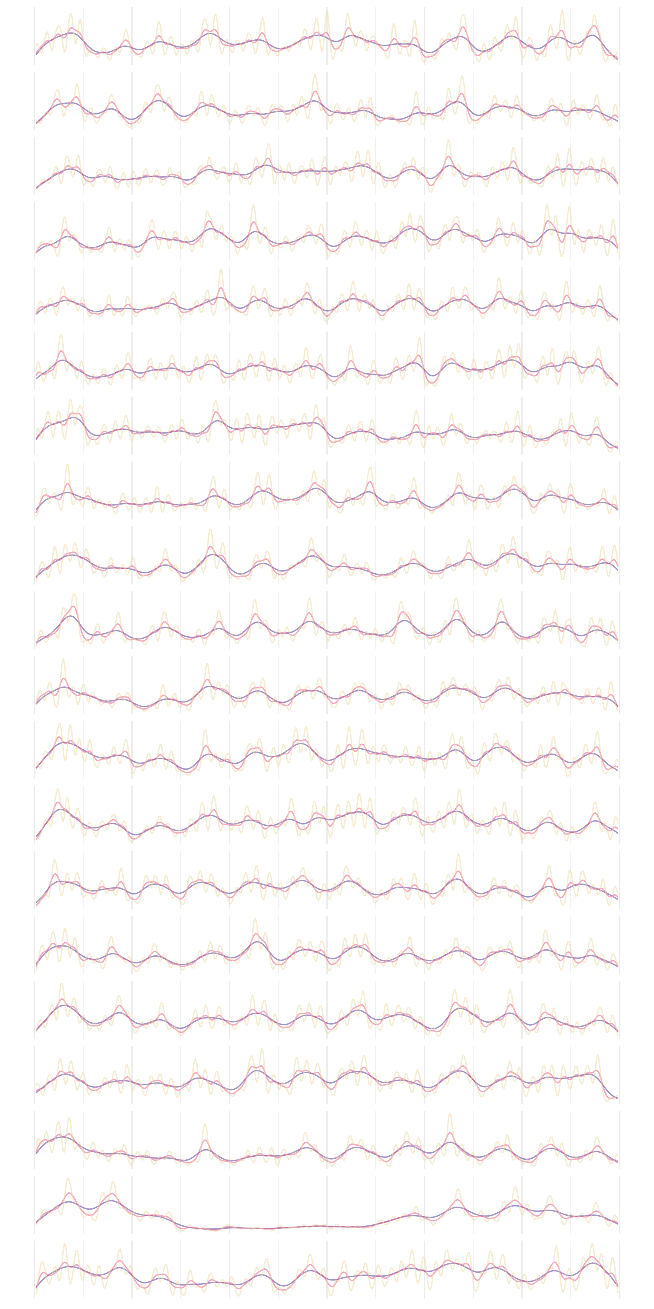
Temporal effects
Coming soon
Conclusions?
Coming soon with the temporal analysis
